Starting from version 2.6.58, facets in Molflow+ can have angle maps. 

Purpose

• You can record the distribution of the incident angles on a facet
• You can desorb gas (i.e. generate outgoing angles) according to a recorded distribution
• You can combine the two modes above: record incident angles on a facet, then use the recorded distribution to generate outgoing angles, either on the same or on a different facet

The two dimensions

• Theta, the incident (elevation) angle: the angle between the incident or outgoing direction and the facet's normal. It is therefore 0 if the direction is perpendicular to the facet's plane, and approaches PI/2 as the direction approaches the facet plane.
• Phi, the azimuth angle: this is the angle between the facet's U vector of the particle direction's projection on the facet plane

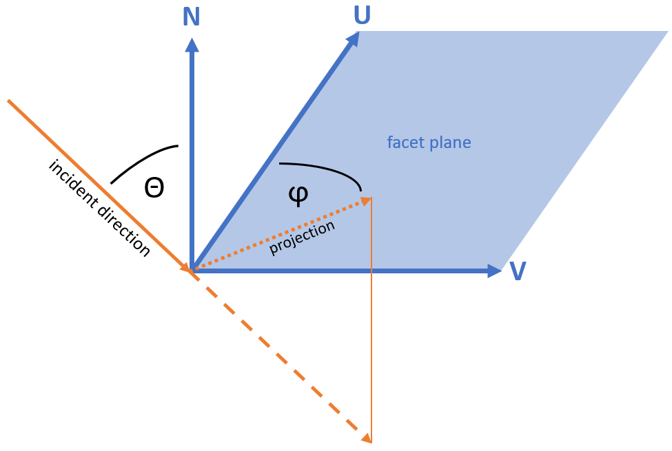
Note: a facet's U vector is its longest side by default, which can be rotated with the Facet / Shift Vertex command. You can visualize the U, V and normal vectors by selecting a facet and enabling these view options through the checkboxes in the upper right corner.

Parameters

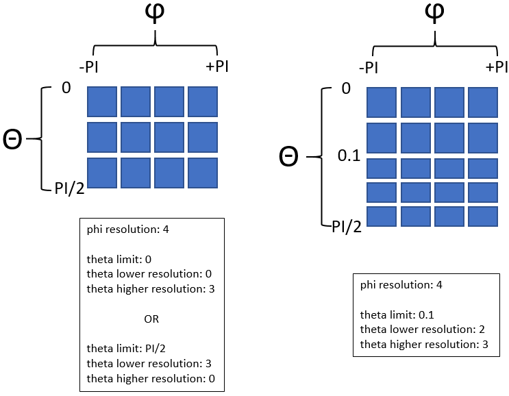
Just like for any one- or two-dimensional distribution, before creating an angle map, we have to decide the resolution. To make things more complicated, there are often situations when - due to beaming effect, for example - most of the incident particles are nearly perpendicular to a facet. Sampling the near-perpendicular part in detail would require to create a very large angle map, most of which would be a waste of space (the non-perpendicular parts). To solve this, the following parameters describe an angle map in Molflow:

• Phi resolution: determines how many bins the azimuth angles are sampled in the possible values of -PI .. +PI
  Example: a phi resolution of 20 would create the following bins: -PI .. -0.9PI, -0.9PI ... -0.8PI, ... , +0.9PI .. +PI
• Theta angle limit [optional]: Splits the 0...PI/2 incident angle range to a low-resolution and a high-resolution part, so the two regions can have different sampling resolutions. If you don't want to split the region, this value can either be 0 or PI/2
  Example: a theta limit of 0.1 would allow to sample the 0..0.1 incident angle part with high resolution, and the 0.1...PI/2 part with a lower resolution
• Theta lower resolution: Determines how many bins are created between 0 and theta angle limit
  Example: With a theta lower limit of 0.1, and a lower resolution of 10, the created bins would be: 0..0.01, 0.01..0.02, ..., 0.09..0.1
• Theta higher resolution [optional]: Determines how many bins are created between theta angle limit and PI/2

Two cases for clarification:

Recording

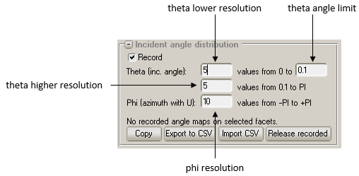
To start collecting incident angles on one or more facets, you have to input these parameters in the Incident angle distribution panel of the Advanced facet parameters window (you might need to expand this panel first):

Note: even if you've enabled the Record checkbox and clicked Apply, the status label will say "No recorded angle maps". This is normal: you have just initialized the map, but the recording will only happen once the subprocesses synchronize with the interface, i.e. when you click Begin.

Important: if you change the angle map parameters (like the resolution), Molflow+ will reinitialize the map - the old recorded map will be overwritten.

Reading a recorded map

Angle maps can be large. Although a dediceated viewer interface withing Molflow is planned, currently the easiest way to read a recorded angle map is copy it to the clipboard and paste it to Excel.

You can optionally use Excel's conditional formatting option to assign color-codes to the cells.

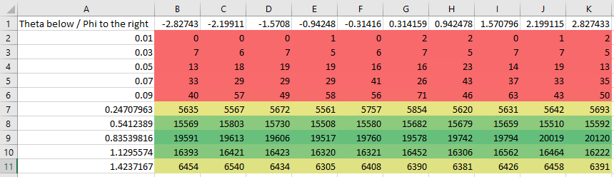
Recorded angle maps pasted to Excel. They correspond to a cosine elevation (theta) distribution, uniform in all azimuth (phi) angles. Click image for full size

Each column belongs to a certain azimuth (phi) angle: the column headers mark the centerpoint (mid-value) of the bins.

Each row belongs to a certain elevation (theta) angle: the values in the first column are therefore the cetnerpoints of the bins. In the example screenshot above, the second row has a header value of 0.03 radians, therefore values in that row show the number of hits between theta=0.02 and theta=0.04 radian incident angles (with the displayed theta=0.03 radians the centerpoint).

Important: there is a difference between the angular distribution in a volume and those sampled on a facet. For this, read section 2.8.0.5 (angular profiles) of the document "The algorithm behind Molflow" on the Molflow documentation page.

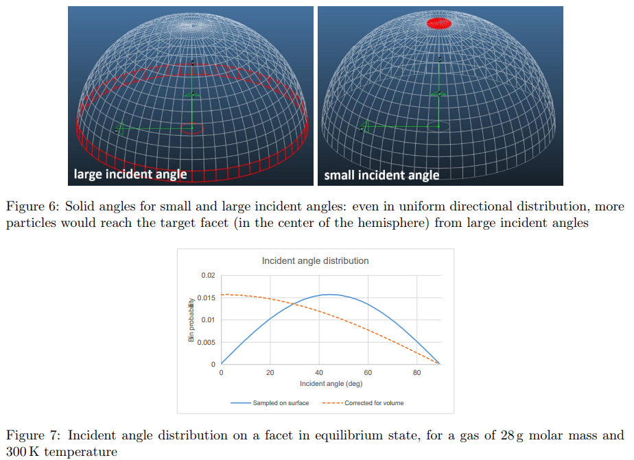
Difference between angular distribution in the gas and sampled on a facet. Click for full size

Exporting angle map(s)

Instead of copying to clipboard, you can select one or more facets and export them to external files. This will allow later to reuse these sampled distributions for particle generation. If you select multiple facets, the filename you specify in the Save As dialog will get a suffix with the facet number. For example, selecting facets 1,5,7 and exporting with the name "distribution" will create three files:

• distribution_facet1.csv
• distribution_facet5.csv
• distribution_facet7.csv

Importing a recorded or custom angle map

Recorded angle maps are saved with Molflow files (when saved in XML or ZIP format). You can, however, import CSV files to any selected facet, therefore you can reuse a recorded angular distribution in a different geometry, or even create your own distribution. If you create your own angle map, the distribution probabilities must be integers, and you can choose between two formats:

Angle map without header

In this case Molflow will assume equal spacing in both directions, so you need to create a simple CSV file where...

• The number of rows is the theta resolution, consequently each row belongs to theta_center= PI/2*(row_index-0.5)/(number_of_rows)
• The number of columns is the phi resolution, consequently each column belongs to phi_center= -PI + 2PI*(column_index-0.5)/(number_of_columns)

​Angle map with headers

Allows to include a theta angle limit (different lower and higher resolutions) and to load exported angle maps directly. The format must strictly match that of the exported files, since Molflow+ has to figure out the angle map parameters (resolution, theta limit, etc.) solely on the header row and the first column values:

• The first row, starting from the second (B1) cell must contain the azimuth (phi) angle centerpoints. It must cover the -PI..PI range and the delta between two values must be constant (equal to the bin width). Consequently, the first value has to be the half bin width, and the last value PI-half_bin_width.
• The first column, starting from the second (A2) cell must contain the elevation (theta) angle centerpoints. They have to be equally spaced, but optionally one delta change is permitted at theta angle limit. It is not necessary to cover the 0...PI/2 period as either the theta lower resolution and theta higher resolution can be zero (no recording below/over the limit).
• The A1 cell can be either empty or start with "Theta" (like "Theta below / Phi to the right")

Valid examples:

• 0.1, 0.3, 0.5 (theta lower resolution: 3, theta angle limit: 0.6, theta higher resolution: 0)
• PI/20, 3PI/20, 5PI/20, 7PI/20, 9PI/20 (theta lower resolution: 5, theta angle limit: PI/2, theta higher resolution: 0)
• 0.1, 0.3, 0.5, 0.7, 0.9, 1.2854 (theta lower resolution: 4, theta angle limit: 1.0, theta higher resolution: 1)

Invalid examples:

• 0.1, 0.3, 0.9 (two spacing breaks would be necessary to cover 0...PI/2)
• 0, 0.1, 0.2 (invalid first value centerpoint)

Important: once again, it is necessary to understand the difference between angular distribution in the gas and on a facet. In general, on a facet, every value is weighed by sin(theta), the solid angle belonging to that elevation. A cosine distribution would therefore be sampled (and generated as) sin(theta)*cos(theta).

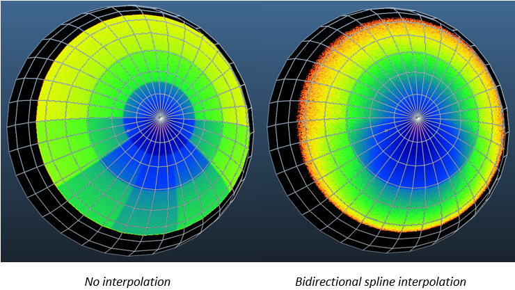
Interpolation

Molflow will perform a weighed spline interpolation in both (phi and theta) directions to create smooth transitions between angle map cells. The azimuth (phi) values are periodic: the angle closest to -PI is interpolated with the angle closest to PI.

Generating according to a recorded angle map

Once a facet has a recorded angle map (either through recording or through importing), set up a desorption by selecting the Recorded angular option and assigning a desorption value (which can optionally be a time-dependent parameter):

Important: you must either record an angle map or use it. When setting up a facet desorption to use the Recorded option, disable the Record checkbox in the advanced parameters, otherwise you'll receive an error:

Switching from recording to generating

If you want to sample the angle map on a facet then immediately generate from it (for example in case of a sequential simulation), it is important to do as follows:

• Set up recording the angle map on the target facet
• Run and Pause the simulation to record the angle map. Optionally save the file
• Do not disable the desorption on the original facet, since that would reset the simulation and clear the recorded angle map. Instead, you'll don it at the next point...
• Disable the recording checkbox on the target facet. Now you can click apply, Molflow will thus recognize that this is a simulation reset where the angle map is to be kept in memory.
• You can set the desorption from the target facet by selecting the Recorded option and assigning an outgasing value and siable the original outgassing.

Sample file using angle map

hemisphere_example.zip

In this example Facet257 in the centre of the hemishpere generates according to the following angle map:

Click for full size

• One azimuth-symmetric row with a peak in the centre for theta=0 to theta=0.6
• One closing circle with 0 values (interpolating with the previous circle) from theta=0.6 to theta=PI/2