There is a Youtube video showing how to use the time-dependent mode in the webinar series.

Since version 2.6 Molflow supports time-dependent simulations. For such, before running the simulation, the user has to define:

• Moments when the system state is sampled. The reason this is necessary is that Molflow is an event-driven simulator, therefore particles are traced individually, looking for the next collision location, and the moment these hits happen is calculated retrospectively. Since a good simulation gathers statistics from possibly millions of hits, it would be impossible to store all of them in memory. Therefore, the user decides the location (through textures/profiles, etc.) and the time (through moments) of the system parts to sample.
  Example: you have a system that reaches its final state during 1s. Therefore you define time moments as 0ms, 100ms, 200ms, ... 1000ms.
• A time window. This defines the duration (or tolerance) during which two hits are considered to happen at the same time. This is necessary as no hits will happen exactly (with perfect precision) at the moments set up above. A too big time window will "smooth out" rapid system changes whereas a too small will require a very long simulation to gather enough statistical data, see below. In practice, most of the time, moments are spread evenly from 0 to steady state, and the time window equals the spacing.
  Example: for the above system, setting a time window of 100ms will make time moments count 0ms..50ms, 50...150ms, ... 950..1050ms respectively.

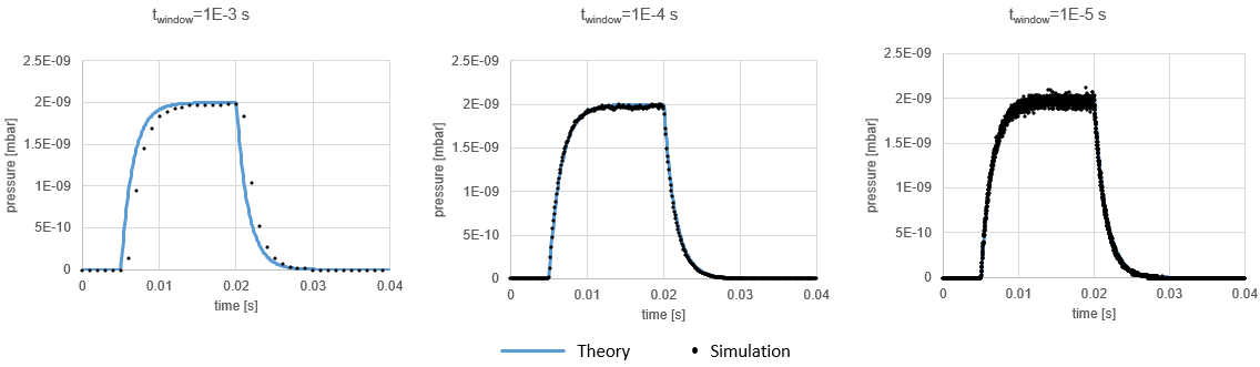
Examples of a pumpup-pumpdown process with too large, normal and too small time windows [click to enlarge]

• Optionally, you can define a time-dependent outgassing through parameters. Many times we are interested in the behavior of a gas pulse after injection, for example. This is optional, though, as even with constant outgassing, the system can change - if we open a valve or start a pump, for example.

Defining moments

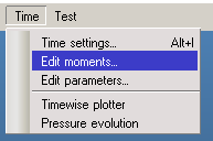
This is done through the Time / Edit moments menu:

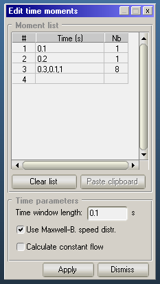
In this window we can define moments in seconds either one by one (as for 0.1s and 0.2s), or through series: 0.3,0.1,1 means eight moments starting from 0.3s, ending at 1s with equal 0.1s spacing.

Hint: don't forget to click outside of the text box after typing - that's when your input is validated and the "Nb" field is filled

In the same window, the time window length field is where you define the tolerance, as described above. In the screenshot it's 0.1s corresponding to the spacing between the moments.

The Use Maxwell-Boltzmann speed distribution option is usually on: if deactivated, molecules will fly with an average speed corresponding to their mass and temperature, instead of the default distributed one.

The Calculate constant flow is an important option, basically asking if we're interested in the system's steady state:

• When on, molecules are traced until pumped. Advantage: the default time moment called "constant flow" is calculated, so the steady state of the system can be queried
• When off, molecules are traced until the last defined moment, i.e. 1s in the example above. The logic is that we're not interested in the steady state of the system, so any hit happening after 1050ms (the last moment and half the time window) will not affect our results. Therefore the particle that passed the last moment is eliminated and a new one is desorbed from source.

When you click apply, the moments will be stored. This also has an important memory implication: every profile, texture, and facet counter will be stored as many times in memory as the number of moments you've defined. Usually you don't want more than 100 moments.

Recalling results

In the Time Settings window (Time / Time Settings or Alt-I) you can choose which moment is displayed.

Textures, profiles, formulas, and counters in the facet hit list (lower right corner) and the Facet Details window all update on the screen as you change the displayed time.

Defining parameters - time-dependent outgassing

Time dependent parameters allow to change the following facet parameters:

• Outgassing
• Sticking
• Opacity

To use them, we give their name instead of a numerical value as the facet parameter. In the example below, we'll set up a pulsed outgassing, so we write an arbitrary name, for example "injection" in the outgassing field:

Then we proceed to define the parameter:

A gas puff defined as a parameter. [Click to enlarge]

For this, we define time-value pairs.

• At the moments we define in this window, the parameter will take the values we assign. Note: these moments are not necessary related to the simulation sampling moments we defined in the first step. These only control the parameter value at different moments.
• Between the defined moments, the value will be linearly interpolated
• Before the first defined moment, the parameter will have the first value (0 in the example above)
• After the last defined moment, the parameter will keep the last value (also 0)

The Plot button draws the curve for verification, whereas the Apply saves the parameter. These parameters are also saved with the simulation file, so they remain when our project is reloaded.