MAG files (with any actual extension, either the default .mag or for example .txt) can provide further information about a magnetic element, that had no place to edit in the GUI.
In MAG files, the separator is whitespace:
- newline(s)
- TAB(s)
- space(s)
- or a mixture of the above
are considered the same.
Local/global components
Change: starting from Synrad version 1.4.31, the MAG files you assign to the Bx, By, Bz components can either mean...
- The global Bx, By, Bz magnetic fields (oriented towards the X,Y,Z global directions). This was the only mode until Synrad 1.4.30
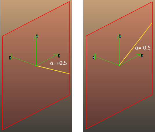
- The local Bx', By' and Bz' magnetic fields, with orientation towards the local X', Y', Z' orthonormal basis (different for every point of the trajectory), determined as:
- Z' points towards the beam (particle) direction, except when using a reference direction (see cases below), in that case it points to the reference direction defined in the first line of the .MAG file.
- Y' towards the global Y axis (accelerators are usually planar and lie in the XZ plane)
- X' computed as a cross product: X'=Y' x Z'. (In the special case of Z'=Y, the X' vector would be a null vector, in that case X'=X)
Constant field
This option does not require a MAG file, values enetered in the GUI will be the Bx,By,Bz or Bx',By',Bz' components.
If choosing the "local coordinates option", the Z' will be the local beam (particle) direction, commonly referred to as S. It also means that Bz' will not bend the beam (Lorentz force is zero as B parallel to v).
Example: simple dipole with target
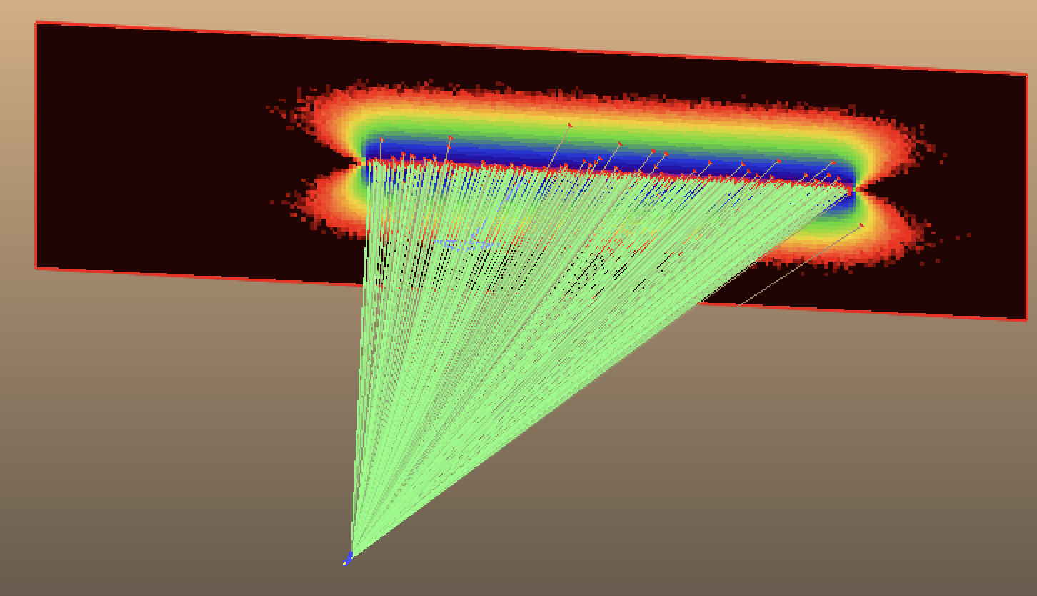
Param file only: simple_dipole.param
With target and textures: simple_dipole_with_target.syn7z
If the magnetic field is not constant, you have 8 different options to define one component of the B vector using a MAG file.
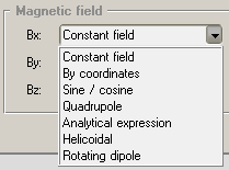
- Coordinates along a direction
- Coordinates along the beam
- Sine / Cosine (i.e. wiggler)
- Quadrupole
- Analytical expression
- Helicoidal
- Rotating dipole
- Combined function magnet
- Curved quadrupole
Coordinates along a direction
The simplest and most often used magnetic field: you define a strength for a list of coordinates, and Synrad will interpolate between them.
MAG file format:
period dirX dirY dirZ N
coordinate1 value1
coordinate2 value2
...
coordinateN valueN
Meaning of the values:
- period: allows you to repeat the values. For example, if period is 50cm, then at 70cm, 120cm, etc... distances Synrad will look up the value at 20cm distance on the reference direction. If you don't want to repeat values, set an arbitrarily large value
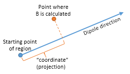
- dirX, dirY, dirZ: the reference direction: starting from the magnetic region's start point a section is defined in the reference direction. At every point in the region, they will be projected to this reference section when looking up coordinates, see drawing below.
- N: number of coordinate-value pairs to follow (required as Synrad doesn't distinguish between whitespaces, numbers can be separated by newline(s), space(s), tab(s) or a combination of these)
- coordinateN valueN pairs: at coordinateN projected distance (in cm) from the starting point of the magnetic region, the magnetic field is valueN (in T)
Typical usage: you have a magnetic element (a dipole, for example) that begins at the starting point of the region, and is orientated in the (dirX,dirY,dirZ) direction.
To calculate the magnetic field strength, the following is done:
1. The actual position is projected to the direction vector (scalar multiplication of the direction vector and the [actual_position-starting_point] vector
2. The projection is interpreted as the "coordinate" (distance) and being looked up in the first column
3. It is interpolated between the N fixed coordinated (distances) written in the lines
If using the "local coordinates" option, Z' is the reference direction (dirX,dirY,dirZ), Y' is Y and X'=Y'xZ'.
Example: Your MAG file is the following for the Bx component:
100.0 0.0 0.0 1.0 2
0 2.0
100.0 3.0
It means the following:
- the period is 100 cm
- oriented towards the global Z axis (0,0,1)
- It has 2 coordinates (two lines) that follow
- At 0cm (beginning) it has 2T field
- At 100cm (end) it has a 3T field
Bx(0,0,50)=2.5Tesla (halfway between the two fixed coordinates)
Bx(0,0,120)=2.2Tesla (The period of 100cm is deducted from the 120cm distance)
The above two calculations assumed that the starting point (defined in the .param file or the Region Editor) is (0,0,0).
Example:
Coordinates along the beam
Use the same format as above. The dirX, dirY, dirZ numbers will be ignored. The coordinate will be the L value (distance along beam), with full periods subtracted.
Sine / cosine (wiggler)
You can define a periodic magnetic field. With one harmonic it is a wiggler. Format of the BXY file:
period dirX dirY dirZ N
A1 B1
A2 B2
...
AN BN
- period is the period of the sine and cosine function
- dirX, dirY and dirZ are the reference direction as described in "coordinates along the direction". This also defines the Z' local vector when "local components" mode is chosen.
- N is the number of lines that follow.
A1, B1, A2, B2, ... are coefficients, to give the following magnetic field:
B(distance)=
A1*sin(distance*2PI/period) + B1*cos(distance*2PI/period) +
A2*sin^2(distance*2PI/period) + B2*cos^2(distance*2PI/period) +
...
AN*sin^N(distance*2PI/period) + BN*cos^N(distance*2PI/period)
For example, a wiggler with a 10cm direction, pointing in the Z (0,0,1) direction, and 0.1T peak field looks like this:
10 0 0 1 1
0.1 0
Quadrupole
If you choose this mode, one component's MAG file will set all the components of the magnetic vector. Load it as the X component's MAG file.
Format of the MAG file:
centerX centerY centerZ
alfa theta rot
K L
(centerX,centerY,centerZ) define where the center point of the beginning of the quadrupole is (ie. the starting point of its axis).
For a "beam on quadrupole axis" scenario, it is the same as the region's starting point. However, it is possible to define an off-axis (bending) quadrupole.
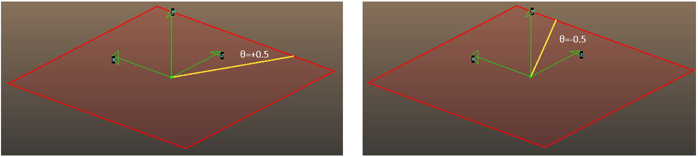
Alfa, theta and rot are 3 angles that define the quadrupole's axis orientation. Careful, the order of alfa and theta is the opposite of the GUI in the region editor. The meaning of the angles, in radians, are:
alpha: angle with the XZ plane, negative towards Y
theta: angle with YZ plane, negative towards X
rot: quadrupole rotation around its centerline (that is defined by alpha, beta). If rot=PI/2, it changes the quad from focusing to defocusing and vica versa.
direction.X= -cos(alpha)*sin(theta)
direction.Y= -sin(alpha)
direction.Z= cos(alpha)*cos(theta)

With the above parameters, you have the starting point and the direction of the axis.
K is the strength of the quadrupole (in Tesla*meters), and L is its length in cm (magnetic field is 0 outside the quadrupole).
You can see the snippet code calculating the quadrupole field here.
Analytic expression
Allows to set up the Halbach wiggler field model.
This mode also sets the B vector's all components. Load the MAG file for the X component! MAG file format:
period dirX dirY dirZ N
Kx K2
Here dirX,dirY, dirZ and N are not used (give any value).
The B vector is calculated the following way:
K=2PI/period
Ky=sqrt(K^2-Kx^2)
Bx(positionX,positionY,positionZ) = Kx/Ky*K2*sinh(Kx*positionX)*sinh(Ky*positionY)*cos(K*positionZ)
By(positionX,positionY,positionZ) = K2*sinh(Kx*positionX)*sinh(Ky*positionY)*cos(K*positionZ)
Bz(positionX,positionY,positionZ) = -K/Ky*K2*sinh(Kx*positionX)*sinh(Ky*positionY)*cos(K*positionZ)
This mode deosn't (yet) support "local components" mode.
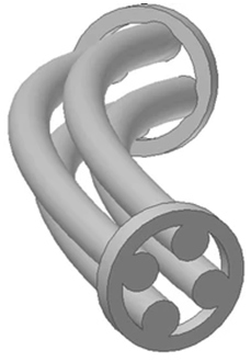
Helicoidal
A helix. MAG file format:
period phase dirX dirY dirZ N
X1 Y1
X2 Y2
...
XN YN
The magnetic component is calculated the following way:
distance = distance along the (dirX,dirY,dirZ) reference direction
ratio = distance*2PI/period
B = X1*sin(ratio)*cos(PI*phase/period) + Y1*cos(ratio)*sin(PI*phase/period)
+ X2*sin(2*ratio)*cos(PI*phase/period) + Y2*cos(2*ratio)*sin(PI*phase/period)
+ ...
+ XN*sin(N*ratio)*cos(PI*phase/period) + YN*cos(N*ratio)*sin(PI*phase/period)
Rotating dipole
Load it as X component, sets all 3 components of the B vector.
MAG file:
period dirX dirY dirZ N
A X
where only period and A have meanings (give any value for others).
ratio = distance*2PI/period
Bx(ratio)=A*sin(ratio)
By(ratio)=A*cos(ratio)
Bz=0
Combined function magnet
Works the same as a quadrupole described above, but a constant magnetic field is added at each point. (Note: the centerline of this quadrupole is still assumed straight. For curved quadrupoles, use there is an other option below)
If you choose this mode, one component's MAG file will set all the components of the magnetic vector for the combined function magnet (CFM). Load it as the X component's MAG file.
Format of the MAG file:
centerX centerY centerZ
alfa beta rot
K L
BXOff BYOff BZOff
(centerX , centerY , centerZ) define where the center point of the beginning of the quadrupole is (i.e. the starting point of its axis).
alfa, beta and rot are 3 angles that define its orientation. The meaning of the angles (in radians) are:
- alpha: angle with the XZ plane, positive towards Y
- beta: angle with YZ plane, negative towards X
- rot: CFM rotation around its centerline (that is defined by alpha, beta). If rot=PI/2, it changes the quad from focusing to defocusing and vica versa.
With the above parameters, you have the starting point and the direction of the axis.
K is the strength of the CFM (in Tesla*meters), and L is its length in cm (magnetic field is 0 outside the CFM).
Additionally, (BXOff , BYOff , BZOff) define an offset to the magnetic field in the CFM's coordinate system.
Curved quadrupole
This is similar to a combined function magnet: it is also a quadrupole that adds a magnetic offset. The difference is that the quadrupole's reference centerline is also curved: it follows the path of a beam particle that would fly in the magnetic offset's field (typically the magnetic offset has a single component and thus the centerline is a dipole's curve).
Every point of the beam is first matched with the closest point on the reference curve (see the steps below how the closest point is determined). Then the quadrupole's magnetic field is calculated in that point's normal plane, and finally the offset is added.
The format of the MAG file is exactly the same as for the combined function magnet:
centerX centerY centerZ
alfa beta rot
K L
BXOff BYOff BZOff
(centerX , centerY , centerZ) define where the center point of the beginning of the quadrupole is (i.e. the starting point of its reference centerline).
alfa, beta and rot are 3 angles that define its initial orientation (at its beginning). The meaning of the angles (in radians) are:
- alpha: angle with the XZ plane, positive towards Y
- beta: angle with YZ plane, negative towards X
- rot: quad rotation around its centerline (that is defined by alpha, beta). If rot=PI/2, it changes the quad from focusing to defocusing and vica versa. The rotation is maintained along the curved centerline.
K is the strength of the quadrupole (in Tesla*meters), and L is its (curved) length in cm (magnetic field is 0 outside the [0,L] range).
(BXOff , BYOff , BZOff) define an offset to the magnetic field in every point of the region, and also define the reference curve, see below.
Here is an overview of the curved quadrupole, and how the magnetic field is determined:
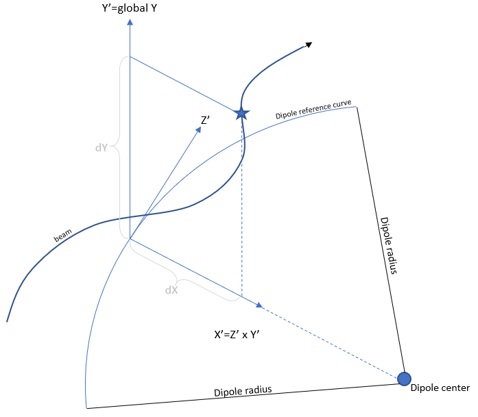
- The curved centerline of the quadrupole is calculated. Its first point is the centerX,centerY,centerZ, its first tangent direction is defined by alpha and beta. The curve is based on the mass, charge and (reference) energy of the particle, and the BXOff BYOff BZOff magnetic offset. In the picture above, only the BYoff component is non-zero, thus the reference curve is that of a horizontally bending dipole. Based on the calculated curve, its center, radius and its bending plane are determined and stored.
- To determine the magnetic field of an arbitrary beam point (star symbol in the picture), it is first projected to the bending plane.
- From the curve center, a line is drawn towards the projected location (on the bending plane). This line will intersect the curve, determining the "closest" point of the curve to the beam point.
- The beam point will be in the normal plane (spanned by X' and Y') of the curve's closest point, determined in the previous step. Its location dX,dY, expressed in X',Y' coordinates, is calculated.
- If the quadrupole is rotated (rot angle non-zero), a 2D rotation (around the curve's tangent) is applied to update dX,dY.
- The quadrupole magnetic field is calculated: By' = K * dX; Bx' = K * dY
- The magnetic field Bx',By' is transformed back to global Bx,By,Bz coordinates.
- The magnetic offset BXOff,BYOff,BZOff is added.